1. 데이터 읽기

• 벡터 데이터 읽기
  • read_file(*.shp) : shp파일 읽어서 geoDataFrame에 저장

import geopandas as gpd
df = gpd.read_file(r'data/MOCT_LINK.shp',encoding='CP949')
df.head()

• Geometry 표시 하기

%matplotlib inline
df.plot(color='black')

2. geoDataFrame 구조 확인

• type 확인

type(df)

geopandas.geodataframe.GeoDataFrame

• row, column 크기 확인

df.shape

(1331, 18)

• column명 확인

df.columns

Index(['LINK_ID', 'F_NODE', 'T_NODE', 'LANES', 'ROAD_RANK', 'ROAD_TYPE',
       'ROAD_NO', 'ROAD_NAME', 'ROAD_USE', 'MULTI_LINK', 'CONNECT', 'MAX_SPD',
       'REST_VEH', 'REST_W', 'REST_H', 'LENGTH', 'REMARK', 'geometry'],
      dtype='object')

• Geometry type 확인

df.geom_type

0         LineString
1         LineString
2    MultiLineString
3         LineString
4         LineString
dtype: object

3. 좌표계 확인

• 좌표계 확인

df.crs

<Projected CRS: PROJCS["ITRF2000_Central_Belt_60",GEOGCS["GCS_ITRF ...>
Name: ITRF2000_Central_Belt_60
Axis Info [cartesian]:
- [east]: Easting (metre)
- [north]: Northing (metre)
Area of Use:
- undefined
Coordinate Operation:
- name: unnamed
- method: Transverse Mercator
Datum: International Terrestrial Reference Frame 2000
- Ellipsoid: GRS 1980
- Prime Meridian: Greenwich

• 좌표계 변경

merc = df.to_crs({'init':'epsg:4326'})
merc.plot(color='black')

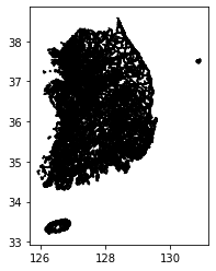
4. 포맷 변환

• GeoDataFrame을 json 포맷으로 변환

# 데이터가 커서 sample로 1개 데이터만 json으로 변환
df.head(1).to_json()

'{"type": "FeatureCollection", "features": [{"id": "0", "type": "Feature", "properties": {"CONNECT": "000", "F_NODE": "2630076801", "LANES": 1, "LENGTH": 1410.19291001225, "LINK_ID": "2630193301", "MAX_SPD": 60, "MULTI_LINK": "0", "REMARK": null, "REST_H": 0, "REST_VEH": "0", "REST_W": 0.0, "ROAD_NAME": "\\ud654\\uc545\\uc0b0\\ub85c", "ROAD_NO": "391", "ROAD_RANK": "106", "ROAD_TYPE": "000", "ROAD_USE": "0", "T_NODE": "2630076901"}, "geometry": {"type": "LineString", "coordinates": [[245889.20842293755, 602540.1031623926], [245884.52438196362, 602550.7076639828], [245880.5845997197, 602562.441661735], [245877.37697640058, 602577.5560817202], [245874.80402102915, 602590.923142394], [245870.08166344027, 602608.6555760134], [245866.14860266628, 602619.1390588756], [245861.72407481138, 602627.9941839982], [245850.47753049707, 602649.6933080491], [245843.77653209324, 602663.2882877537], [245840.21593625328, 602674.2739925202], [245836.2741359605, 602686.3831435101], [245833.96002093932, 602698.125878997], [245831.74675705165, 602714.3711385361], [245830.48617608764, 602739.5004281478], [245829.72781690946, 602764.257252305], [245829.78834916753, 602799.523103117], [245829.18865190083, 602818.0280274062], [245827.4648357864, 602836.2767985966], [245825.86203727854, 602855.2765506067], [245823.64944289793, 602871.396758187], [245821.52694263405, 602894.0203128068], [245820.4236764545, 602913.1478050507], [245821.58007512547, 602930.6617291515], [245823.60645547815, 602949.1807706261], [245825.40895076204, 602962.8214614922], [245826.09405003514, 602974.9554847644], [245825.65368618732, 602987.0834576795], [245823.97894215182, 602996.2034733664], [245820.42842643222, 603005.3134050232], [245811.20958754103, 603022.0212222983], [245803.40463366537, 603031.6085023026], [245795.35831640614, 603039.5687689325], [245779.41022924686, 603051.8634824678], [245761.20651050736, 603065.0214546616], [245744.9962197665, 603079.5657484786], [245711.8058337661, 603112.2767922183], [245676.3322525288, 603150.9782006346], [245664.11688441734, 603166.7945190094], [245654.27749311822, 603182.6236104805], [245646.6896994245, 603198.3397514643], [245641.49132830047, 603211.5676374831], [245635.8969615895, 603228.67010031], [245632.192484073, 603243.1565677221], [245627.70139361764, 603264.3917775303], [245625.5082893798, 603276.885489703], [245622.31073984868, 603290.1241318531], [245618.2163164351, 603307.3597129482], [245615.66553742788, 603316.6000712622], [245612.62396502416, 603324.0870205313], [245606.79428443874, 603338.4370064927], [245600.21765677864, 603352.1577013484], [245595.16584919338, 603361.384613071], [245585.18325133767, 603380.5894169775], [245577.72319553196, 603395.8060218558], [245572.39439199885, 603410.0336447023], [245567.3082955352, 603425.6381774854], [245563.35505705074, 603439.873195574], [245557.6094144114, 603461.851987991], [245552.1448012958, 603478.0797602631], [245546.8139796491, 603492.6825364484], [245543.12428970283, 603504.4178705714], [245537.91112339962, 603520.3968842088], [245527.91978245924, 603541.2273534045], [245501.14465575287, 603590.2300162113], [245479.78640583853, 603631.8835551282], [245454.11186099224, 603685.5191653903], [245430.8179966427, 603738.292187912], [245408.38805921804, 603793.195787896], [245399.2431610517, 603819.4081672801]]}}]}'

• GeoDataFrame을 json 파일로 저장
  • driver : 출력 파일 포맷

df.to_file(driver='GeoJSON', filename='link.geojson')

• 파일 출력 시 가능한 포맷
  • GeoPandas는 Fiona 라이브러리를 이용해 출력
  • 아래 명령을 통해 Fiona에서 지원하는 모든 driver 확인 가능

import fiona
fiona.supported_drivers

5. 데이터 다루기

• 첫 번째 데이터 확인

df.loc[0]

LINK_ID                                              2180383101
F_NODE                                               2180132301
T_NODE                                               2180132201
LANES                                                         1
ROAD_RANK                                                   101
ROAD_TYPE                                                   000
ROAD_NO                                                      17
ROAD_NAME                                              서울문산고속도로
ROAD_USE                                                      0
MULTI_LINK                                                    0
CONNECT                                                     101
MAX_SPD                                                      50
REST_VEH                                                      5
REST_W                                                        0
REST_H                                                        0
LENGTH                                                  169.152
REMARK                                                     None
geometry      LINESTRING (310943.9252600061 4166093.43858687...
Name: 0, dtype: object

• 특정 컬럼 데이터 조회

df['ROAD_NAME']

0       서울문산고속도로
1         개화동로8길
2         개화동로8길
3            당산길
4              -
          ...
1326    서울문산고속도로
1327    서울문산고속도로
1328    서울문산고속도로
1329    서울문산고속도로
1330    서울문산고속도로
Name: ROAD_NAME, Length: 1331, dtype: object

• 컬럼 필터링

서울문산고속도로 = df[df['ROAD_NAME'] == '서울문산고속도로']
서울문산고속도로

• Geometry 보기

서울문산고속도로.plot(figsize=(7,7))

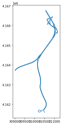
6 공간 Join

• 서울시에 포함되는 Link 찾기 예제
  • 행정경계는 여기에서 다운로드 가능

df2 = gpd.read_file(r'data/TL_SCCO_CTPRVN.shp')
df2.plot()

seoul_link = gpd.sjoin(df, seoul, op='within')

참고

• 파이썬을 활용한 지리공간 분석 마스터하기
• 예제는 국가표준노드링크로 진행

1. Shapely로 Geometry 생성하기

• Polygon 생성하기(튜플)

from shapely.geometry import Polygon
p1 = Polygon(((1,2), (5,3), (5,7), (1,9), (1,2)))
p1

p2 = Polygon(((6,6), (7,6), (10,4), (11,8), (6,6)))
p2

• Point생성하기(좌표값)

from shapely.geometry import Point
point = Point(2.0, 2.0)
point

• Line 생성하기

from shapely.geometry import LineString
line = LineString([(0,0), (10,10)])
line

• Linear Ring 생성하기

from shapely.geometry.polygon import LinearRing
ring = LinearRing([(0,0), (3,3), (3,0)])
ring

• MultiPoint 생성하기

from shapely.geometry import MultiPoint
points = MultiPoint([(0,0), (3,3)])
points

• MultiLine 생성하기

from shapely.geometry import MultiLineString
coords = MultiLineString([((0,0), (1,1)),((-1,0), (1,0))])
coords

• MultiPolygon 생성하기

from shapely.geometry import MultiPolygon
polygons = MultiPolygon([p1,p2])
polygons

2. Shapely 공간 함수

# 면적 구하기
print(p1.area)
# 경계 구하기
print(p1.bounds)
# 길이 구하기
print(p1.length)
# geometry Type 구하기
print(p1.geom_type)

22.0
(1.0, 2.0, 5.0, 9.0)
19.59524158061724
Polygon

3. Shapely로 JSON Geometry 읽기

• Json 파일 생성 및 shape를 이용해 로딩

import json
from shapely.geometry import mapping, shape
jData = json.loads('{"type":"Polygon","coordinates":[[[1,1],[1,3],[3,3]]]}')
p = shape(jData)
p

• geometry를 json형태로 변환

mapping(p)

{'type': 'Polygon', 'coordinates': (((1.0, 1.0), (1.0, 3.0), (3.0, 3.0), (1.0, 1.0)),)}

4 Fiona 데이터 읽기

• shp 파일 정보 표출

print(len(c))
print(c.driver)
print(c.crs)

100
ESRI Shapefile
{'proj': 'tmerc', 'lat_0': 38, 'lon_0': 127, 'k': 1, 'x_0': 200000, 'y_0': 600000, 'ellps': 'GRS80', 'units': 'm', 'no_defs': True}

• shp 파일 데이터 읽기

import fiona
c = fiona.open(r'data/node.shp')
rec = next(iter(c))
print('keys = ', rec.keys())
print('type = ', rec['type'])
print('prop = ', rec['properties'])
print('id   = ', rec['id'])
print('geom = ', rec['geometry'])

keys =  dict_keys(['type', 'id', 'properties', 'geometry'])
type =  Feature
prop =  OrderedDict([('NODE_ID', '1100025100'), ('NODE_TYPE', '101'), ('NODE_NAME', '하계5,6단지앞교차로'), ('TURN_P', '1'), ('REMARK', None)])
id   =  0
geom =  {'type': 'Point', 'coordinates': (205838.0880999937, 559449.3750999967)}

5 데이터 다루기

• shape file 읽고 첫 번째 Feature 정보 가져오기

import fiona
with fiona.open(r'data/node.shp') as src:
    print(src[0])

{'type': 'Feature', 'id': '0', 'properties': OrderedDict([('NODE_ID', '1100025100'), ('NODE_TYPE', '101'), ('NODE_NAME', '하계5,6단지앞교차로'), ('TURN_P', '1'), ('REMARK', None)]), 'geometry': {'type': 'Point', 'coordinates': (205838.0880999937, 559449.3750999967)}}

참고

• 파이썬을 활용한 지리공간 분석 마스터하기
• 예제는 국가표준노드링크로 진행

1. OGR 라이브러리

• OGR의 3가지 Component
  • OGR 배치 명령 : 벡터 데이터 정보 요약 및 변환
  • 파이썬 스크립트 : 미리 개발해 놓은 GIS 분석 기능
  • OGR 라이브러리 : 파이썬에서 사용할 수 있는 OGR 라이브러리

2. OGR 배치 명령

• OGR은 벡터데이터 요약 정보 제공, 변환 등을 위한 배치 명령을 제공
• 대표적으로 아래와 같은 배치 명령 존재
  • ogrinfo : 벡터 데이터 요약정보 확인
  • ogr2ogr : 벡터 파일을 다른 포맷으로 변경
  • ogrtindex : 벡터 타일 생성
  • ogr2vrt : 벡터 타일 생성(orgtindex 보다 광범위하게 사용됨)
• 터미널에서 명령을 수행함
  • Jupyter notebook에서 명령어 앞에 !를 붙이면 터미널 명령 수행 가능

2.1 ogrinfo

• 파일 입출력 가능 포맷 조회

!ogrinfo --formats

Supported Formats:
...
  ESRI Shapefile -vector- (rw+v): ESRI Shapefile
  KML -vector- (rw+v): Keyhole Markup Language (KML)
  GeoJSON -vector- (rw+v): GeoJSON
...

• 파일의 요약 정보 보기
  • data 폴더의 link 파일 요약 정보 보기
  • -so : 요약 정보만 보겠다는 옵션
  • -so가 없으면 shp의 모든 정보를 표시함

!ogrinfo -so "data" MOCT_LINK

INFO: Open of `data'
      using driver `ESRI Shapefile' successful.

Layer name: MOCT_LINK
Metadata:
  DBF_DATE_LAST_UPDATE=2021-03-30
Geometry: Line String
Feature Count: 528232
Extent: (101766.537600, 67516.493200) - (546275.776100, 665746.517600)
Layer SRS WKT:
PROJCS["ITRF2000_Central_Belt_60",
    GEOGCS["GCS_ITRF_2000",
        DATUM["International_Terrestrial_Reference_Frame_2000",
            SPHEROID["GRS 1980",6378137,298.257222101,
                AUTHORITY["EPSG","7019"]],
            AUTHORITY["EPSG","6656"]],
        PRIMEM["Greenwich",0],
        UNIT["Degree",0.0174532925199433]],
    PROJECTION["Transverse_Mercator"],
    PARAMETER["latitude_of_origin",38],
    PARAMETER["central_meridian",127],
    PARAMETER["scale_factor",1],
    PARAMETER["false_easting",200000],
    PARAMETER["false_northing",600000],
    UNIT["metre",1,
        AUTHORITY["EPSG","9001"]],
    AXIS["Easting",EAST],
    AXIS["Northing",NORTH]]
Data axis to CRS axis mapping: 1,2
LINK_ID: String (10.0)
F_NODE: String (10.0)
T_NODE: String (10.0)
LANES: Integer (4.0)
ROAD_RANK: String (3.0)
ROAD_TYPE: String (3.0)
ROAD_NO: String (5.0)
ROAD_NAME: String (30.0)
ROAD_USE: String (1.0)
MULTI_LINK: String (1.0)
CONNECT: String (3.0)
MAX_SPD: Integer (4.0)
REST_VEH: String (3.0)
REST_W: Integer (4.0)
REST_H: Integer (4.0)
LENGTH: Real (18.12)
REMARK: String (30.0)

• KML 파일 읽기
  • 샘플 데이터 : 다운로드

!ogrinfo "KML_Sample.kml" -summary

INFO: Open of `KML_Sample.kml'
      using driver `KML' successful.
1: Placemarks (3D Point)
2: Highlighted Icon (3D Point)
3: Paths (3D Line String)
4: Google Campus (3D Polygon)
5: Extruded Polygon (3D Polygon)
6: Absolute and Relative (3D Polygon)

2.2 ogr2ogr

• shp 파일을 GeoJson파일로 변환

!ogr2ogr -f "GeoJson" "output.json" "data/MOCT_LINK.shp"

3. 파이썬 스크립트

• GDAL 설치 경로에 GIS 분석에 사용할 수 있는 스크립트 제공
  • 경로 예시(anaconda일 때) : C:\Users\82103\Anaconda3\envs\geospatial\Lib\site-packages\GDAL-3.0.2-py3.6-win-amd64.egg-info\scripts
• scripts 예시
  • ogrmerge.py : shp파일을 merge 하여 다른 파일로 변환함
• 사용 방법
  • 터미널 또는 Jupyter notebook에서 사용 방식에 따라 명령 수행

#경로 이동
cd "C:\Users\82103\Anaconda3\envs\geospatial\Lib\site-packages\GDAL-3.0.2-py3.6-win-amd64.egg-info\scripts"

#터미널에서 수행 할 때
ogrmerge.py -f GPKG -o merged.gpkg "MOCT_LINK.shp"

# Jupyter Note Book에서 수행할 때
%run ogrmerge.py -f GPKG -o merged.gpkg "MOCT_LINK.shp"

• 참고 : %run
  • Jupyter notebook의 매직명령
  • 외부 스크립트를 Jupyter notebook에서 실행 할 때 사용

4. OGR 라이브러리

• OGR 라이브러리는 2개의 주요 모듈로 구성
  • ogr : 벡터 지오메트리를 주로 다룸
  • osr : 투영에 관해 다룸
• OGR 이 제공하는 7개의 클래스
  • Geometry : 기하학 좌표 연산/변환 제공, Spatial Reference System을 포함
  • Spatial Reference : 투영과 좌표계 관련 기능 정의
  • Feature : Geometry와 속성정보를 가진 Feature를 정의(Polygon 등의 객체)
  • Feature Class Definition : Feature의 스키마 정보를 정의
  • Layer : Feature들을 모아놓은 Layer 정의
  • Dataset : OGRLayer 객체를 하나 이상 포함하는 File 또는 Database을 표현
  • Drivers : 포맷 변환을 정의하며, 모든 Drivers는 GDALDriverManager에서 관리함

4.1 OGR로 객체 생성하기

• OGR로 Point, Line, Polygon과 같은 벡터 Geometry 생성 가능
• Polygon 생성 예제

from osgeo import ogr
r = ogr.Geometry(ogr.wkbLinearRing)
r.AddPoint(1,1)
r.AddPoint(5,1)
r.AddPoint(5,5)
r.AddPoint(1,5)
r.AddPoint(1,1)
poly = ogr.Geometry(ogr.wkbPolygon)
poly.AddGeometry(r)
print(poly.ExportToWkt())

POLYGON ((1 1 0,5 1 0,5 5 0,1 5 0,1 1 0))

4.2 GeoJSON으로 부터 객체 생성하기

• GeoJSON 구조로 부터 객체 생성 가능
• GeoJSON으로 부터 Polygon 생성 예제

from osgeo import ogr
geojson = """{"type":"Polygon","coordinates":[[[1,1],[5,1],[5,5],[1,5],[1,1]]]}"""
polygon = ogr.CreateGeometryFromJson(geojson)
print(polygon)

POLYGON ((1 1,5 1,5 5,1 5,1 1))

4.3 Geometry 연산 수행

• Polygon Geometry 연산 수행

# 1. 면적 구하기
print("폴리곤 면적은 ", polygon.Area(), "입니다.")

# 2. 중심점 구하기
cen = polygon.Centroid()
print(cen)

# 3. 경계 구하기
boundary = polygon.GetBoundary()
print(boundary)

# 4. Point 가 Polygon 내부에 존재하는지 확인
point = ogr.Geometry(ogr.wkbPoint)
point.AddPoint(10, 10)
polygon.Contains(point)

# 5.  Buffer 구하기
buffer = polygon.Buffer(2)

폴리곤 면적은  16.0 입니다.
POINT (3 3)
LINESTRING (1 1,5 1,5 5,1 5,1 1)
False

4.4 Shape 파일에 Polygon Data 쓰기

• 아래 순서로 진행
  • 좌표계 설정
  • Shape file 생성
  • Layer 생성
  • feature 생성 및 Geometry 입력
  • Layer에 Feature 입력

import osgeo.ogr, osgeo.osr

# 1. 좌표계 설정
spatialReference = osgeo.osr.SpatialReference()
spatialReference.ImportFromProj4('+proj=longlat +ellps=WGS84 +datum=WGS84 +no_defs')

# 2. ShapeFile 생성
driver = osgeo.ogr.GetDriverByName('ESRI ShapeFile')
shapeData = driver.CreateDataSource('polygon.shp')

# 3. layer 생성
layer = shapeData.CreateLayer('polygon_layer', spatialReference, osgeo.ogr.wkbPolygon)
layerDefinition = layer.GetLayerDefn()

# 4. Feature 생성 및 Geometry 입력
featureIndex = 0
feature = osgeo.ogr.Feature(layerDefinition)
feature.SetGeometry(polygon)
feature.SetFID(featureIndex)

# 5. Layer에 Feature 입력
layer.CreateFeature(feature)

# 6. 생성 확인
!ogrinfo polygon.shp

INFO: Open of `polygon.shp'
      using driver `ESRI Shapefile' successful.
1: polygon (Polygon)

4.5 feature 다루기

• Shape 파일을 읽어 특정 필드명 출력

from osgeo import ogr
import os
shapefile = r'data/node.shp'
driver = ogr.GetDriverByName("ESRI Shapefile")
dataSource = driver.Open(shapefile,0)
layer = dataSource.GetLayer()

# 데이터가 많아서 Sample로 5개 필드만 출력
idx = 0
for feature in layer:
    print(idx, ", ", feature.GetField("NODE_NAME"))
    idx += 1
    if(idx == 5):
        break

0 ,  하계5,6단지앞교차로
1 ,  공릉터널남측
2 ,  미성아파트5동앞
3 ,  유토피아빌딩
4 ,  청구빌라4단지401동

• Shape 파일의 모든 필드 이름 나열하기

from osgeo import ogr
source = ogr.Open(r'data/MOCT_LINK.shp')
layer = source.GetLayer()
schema = []
ldefn = layer.GetLayerDefn()
for n in range(ldefn.GetFieldCount()):
    fdefn = ldefn.GetFieldDefn(n)
    schema.append(fdefn.name)
print(schema)

['LINK_ID', 'F_NODE', 'T_NODE', 'LANES', 'ROAD_RANK', 'ROAD_TYPE', 'ROAD_NO', 'ROAD_NAME', 'ROAD_USE', 'MULTI_LINK', 'CONNECT', 'MAX_SPD', 'REST_VEH', 'REST_W', 'REST_H', 'LENGTH', 'REMARK']

• Feature 개수 구하기

from osgeo import ogr
import os
shapefile = r'data/MOCT_LINK.shp'
driver = ogr.GetDriverByName("ESRI Shapefile")
dataSource = driver.Open(shapefile, 0)
layer = dataSource.GetLayer()
featureCount = layer.GetFeatureCount()
print("count = ", featureCount)

count =  528232

4.6 좌표계 다루기

• CRS 정보 조회하기
  • Layer로부터 구하기
  • Geometry로부터 구하기

# 1) Layer로부터 구하기
spatialRef = layer.GetSpatialRef()
print(spatialRef)

PROJCS["ITRF2000_Central_Belt_60",
    GEOGCS["GCS_ITRF_2000",
        DATUM["International_Terrestrial_Reference_Frame_2000",
            SPHEROID["GRS 1980",6378137,298.257222101,
                AUTHORITY["EPSG","7019"]],
            AUTHORITY["EPSG","6656"]],
        PRIMEM["Greenwich",0],
        UNIT["Degree",0.0174532925199433]],
    PROJECTION["Transverse_Mercator"],
    PARAMETER["latitude_of_origin",38],
    PARAMETER["central_meridian",127],
    PARAMETER["scale_factor",1],
    PARAMETER["false_easting",200000],
    PARAMETER["false_northing",600000],
    UNIT["metre",1,
        AUTHORITY["EPSG","9001"]],
    AXIS["Easting",EAST],
    AXIS["Northing",NORTH]]

# 2) Geometry로부터 구하기
feature = layer.GetNextFeature()
geom = feature.GetGeometryRef()
spatialRef2 = geom.GetSpatialReference()
print(spatialRef2)

PROJCS["ITRF2000_Central_Belt_60",
    GEOGCS["GCS_ITRF_2000",
        DATUM["International_Terrestrial_Reference_Frame_2000",
            SPHEROID["GRS 1980",6378137,298.257222101,
                AUTHORITY["EPSG","7019"]],
            AUTHORITY["EPSG","6656"]],
        PRIMEM["Greenwich",0],
        UNIT["Degree",0.0174532925199433]],
    PROJECTION["Transverse_Mercator"],
    PARAMETER["latitude_of_origin",38],
    PARAMETER["central_meridian",127],
    PARAMETER["scale_factor",1],
    PARAMETER["false_easting",200000],
    PARAMETER["false_northing",600000],
    UNIT["metre",1,
        AUTHORITY["EPSG","9001"]],
    AXIS["Easting",EAST],
    AXIS["Northing",NORTH]]

참고

• 파이썬을 활용한 지리공간 분석 마스터하기
• GDAL Vector Data Model
• 예제는 국가표준노드링크로 진행

1. 벡터 데이터 타입

2.래스터 데이터 타입

1. postgresql 설치(postGIS 포함)

• programmerpsy.tistory.com/94

2. 파이썬에서 PostgreSQL 연결하기

• psycopg2 설치하기

conda install -c anaconda psycopg2

3. 데이터 베이스 연결하기

• geospatial DB에 연결 후 points 테이블 생성하는 예제

import psycopg2, pprint

connection = psycopg2.connect(database="geospatial", user="postgres", password="******")
cursor = connection.cursor()

cursor.execute("CREATE TABLE points (id SERIAL PRIMARY KEY, name VARCHAR(255), location GEOMETRY)")
connection.commit()

• psycopg2.connect
  • 데이터베이스명, 사용자ID, PW를 입력하여 DB에 연결
• connection.cursor
  • 데이터베이스와 통신할 수 있는 cursor 생성
• cursor.execute
  • 인자로 입력된 SQL문을 실행
• connection.commit
  • 변경 내용을 DB에 저장

4. 테이블에 데이터 추가

• WKT형태의 좌표를 Geometry로 저장

cursor.execute("INSERT INTO points (name, location) VALUES ('p1',ST_GeomFromText('POINT(100 200)'))")             
cursor.execute("INSERT INTO points (name, location) VALUES ('p1',ST_GeomFromText('POINT(200 400)'))")
cursor.execute("INSERT INTO points (name, location) VALUES ('p1',ST_GeomFromText('POINT(700 300)'))")
cursor.execute("INSERT INTO points (name, location) VALUES ('p1',ST_GeomFromText('POINT(400 300)'))")
cursor.execute("INSERT INTO points (name, location) VALUES ('p1',ST_GeomFromText('POINT(100 400)'))")
cursor.execute("INSERT INTO points (name, location) VALUES ('p1',ST_GeomFromText('POINT(100 300)'))")
connection.commit() 

cursor.execute("SELECT * from points") 
cursor.fetchall() 

• WKT 대신 shapely를 이용해 geometry를 컨트롤 하는 방법
  • shapely의 Point 객체이용
  • Point 객체는 wkt 함수를 이용해 WKT로 변환 가능

from shapely.geometry import Point, MultiPoint
p = [Point(100,200), Point(100,100)]
for pp in p:
    s = ("INSERT INTO points (name, location) VALUES ('p1',ST_GeomFromText('{}'))").format(pp.wkt)
    cursor.execute(s)
connection.commit() 

cursor.execute("SELECT * from points") 
cursor.fetchall() 

• 주피터 노트북에서 이미지 띄우기
  • 좌표 리스트들이 표시됨

MultiPoint(p)

5. 테이블 조회

• points를 조회 하는 예제
  • fetchall() 을 이용하면 select 된 모든 데이터 가져옴
  • fetchone을 이용하면 1개의 데이터만 가져옴

cursor.execute("SELECT * from points") 
data=cursor.fetchall() 
data

[(1, 'p1', '010100000000000000000059400000000000006940'),
 (2, 'p1', '010100000000000000000069400000000000007940'),
 (3, 'p1', '01010000000000000000E085400000000000C07240'),
 (4, 'p1', '010100000000000000000079400000000000C07240'),
 (5, 'p1', '010100000000000000000059400000000000007940'),
 (6, 'p1', '010100000000000000000059400000000000C07240'),
 (8, 'p1', '010100000000000000000059400000000000006940'),
 (9, 'p1', '010100000000000000000059400000000000005940')]

• geomtery가 WKB 형태로 출력
  • shapely를 이용해 WKB-> Point -> WKT 변환 하기

from shapely.wkb import loads
aPoint=loads(data[0][2],hex=True) 
aPoint.wkt

'POINT (100 200)'

6. 좌표계 설정/변경하기

cursor.execute("SELECT UpdateGeometrySRID('points','location',4326)") 
cursor.execute("SELECT Find_SRID('public','points','location')") 
cursor.fetchall()

cursor.execute("SELECT code, ST_AsTexT(ST_Transform(location,3857)) from points") 
cursor.fetchone()

• updateGeomterySRID
  • Geometry에 좌표계 설정함
• Find_SRID
  • Geomtery가 어떤 좌표계 인지 보여줌
• ST_Transform
  • 좌표계를 변경함

7. KNN을 이용한 지정한 점에 가장 가까운 3개 점 얻기

cursor.execute("SELECT name, ST_Distance(location::geography, ST_GeometryFromText('POINT(-106.591838300225 35.1555000000615)')::geography) as d from points ORDER BY location<->ST_GeometryFromText('POINT(-106.591838300225 35.1555000000615)') LIMIT 3") 
cursor.fetchall() 

[('p1', 7120405.75751067),
 ('p1', 16921336.66007583),
 ('p1', 16921336.66007583)]

8. line 데이터 다루기

• line 생성 예제

from shapely.geometry import LineString 
from shapely.geometry import MultiLineString
connection = psycopg2.connect(database="geospatial",user="postgres",password="****")
cursor = connection.cursor() 
cursor.execute("CREATE TABLE lines (id SERIAL PRIMARY KEY, location GEOMETRY)") 
thelines=[] 
thelines.append(LineString([(-106.635585,35.086972),(-106.621294,35.124997)])) 
thelines.append(LineString([(-106.498309,35.140108),(-106.497010,35.069488)])) 
thelines.append(LineString([(-106.663878,35.106459),(-106.586506,35.103979)]))
mls=MultiLineString([((-106.635585,35.086972),(-106.621294,35.124997)),((-106.498309,35.140108),(-106.497010,35.069488)),((-106.663878 ,35.106459),(-106.586506,35.103979))])
for a in thelines:    
    cursor.execute("INSERT INTO lines (location) VALUES (ST_GeomFromText('{}'))".format(a.wkt)) 
    connection.commit() 
cursor.execute("SELECT id, ST_AsTexT(location) from lines") 
data=cursor.fetchall() 
data
connection.commit()

• 두 선 교차 여부 확인 하기
  • ST_Intersects 함수 사용

cursor.execute("SELECT ST_Intersects(l.location::geography,ll.location::geometry) FROM lines l, lines ll WHERE l.id=1 AND ll.id=3") 
cursor.fetchall()

• 두 선을 교차하는 점 확인 하기

cursor.execute("SELECT ST_AsText(ST_Intersection(l.location::geography, ll.location::geometry)) FROM lines l, lines ll WHERE l.id=1 AND ll.id=3") 
cursor.fetchall()

9.Polygon 데이터 다루기

• polygon 생성 예제

  from shapely.geometry import Polygon
  connection = psycopg2.connect(database="pythonspatial",user="postgres", password="postgres") 
  cursor = conectionn.cursor() 
  cursor.execute("CREATE TABLE poly (id SERIAL PRIMARY KEY, location GEOMETRY)") 
  a=Polygon([(-106.936763,35.958191),(-106.944385,35.239293),(-106.452396,35.281908),(-106.407844,35.948708)]) 
  cursor.execute("INSERT INTO poly (location) VALUES (ST_GeomFromText('{}'))".format(a.wkt)) 
  connection.commit()

• 포인트가 폴리곤 내부에 있는지 확인

  • ST_Intersects 또는 ST_Contains 사용

# 참고

• 파이썬을 활용한 지리공간 분석 마스터하기
• WKB, WKT의 이해 및 변환

1. GDAL/OGR

• GDAL 과 OGR 이란?
  • GDAL(Geospatial Data Abstraction Library : 래스터 데이터 처리에 많이 사용하는 라이브러리
  • OGR : 벡터 포맷 데이터 처리에 많이 사용하는 라이브러리
• GDAL 설치 하기
  • 아나콘다 내비게이터를 이용해 설치
    • 가상 환경 생성
    • 생성된 가상환경에 Not installed 설정 -> gdal 검색하여 체크 -> Apply
    • 
  • 아나콘다 프롬프트를 이용해 설치
    • 가상 환경 생성

conda create -n geospatial
activate geospatial
conda install gdal

2. GEOS(Geometry Engine Open Source)

• GEOS란?
  • JTS(Java Topology Suite)의 서브셋과 선택된 기능의 C/C++ 포트
  • JTS의 완전한 기능을 C++로 포함하는 것을 목표
  • QGIS, PostGIS 등 여러 어플리케이션에서 사용됨
  • GDAL과 함께 컴파일해서 OGR의 모든 기능을 제공
• JTS란?
  • Java로 작성된 지리공간 지오메트리 라이브러리
• GEOS 설치하기

conda install -c conda-forge geos

3. Shapely

• Shapely란?
  • 평면 형상의 처리와 분석을 위한 파이썬 패키지
  • GEOS 라이브러리 및 JTS 포트의 기능을 사용함
  • 지오메트리 분석만 다룸(공간 파일을 읽고 쓸 수 있는 기능 없음)
  • 8가지 기본 지오메트리 타입 지원
    • 포인트, 멀티 포인트, 멀티 라인 스트링, 멀티 폴리곤, 폴리곤, 다원형, 지오메트리 컬렉션
  • OGR보다 더 파이썬에 가깝고 직관적인 인터페이스, 최적화가 잘 되어 있음
• Shapely 설치하기

conda install -c scitools shapely

4. Fiona

• Fiona란?
  • OGR API로 데이터 포맷을 읽고 쓰는데 사용
  • OGR 보다 파이썬에 가깝고 신뢰성이 높고 오류 발생률이 낮아 OGR대신 사용
  • 벡터 데이터에 관한 공간 정보를 표현하기 위해 WKT와 WKB라는 두 개의 마크업 언어 사용
  • Shapely와 같은 다른 파이썬 라이브러리와 잘 결합됨
  • 벡터 데이터 복사 시 메모리를 많이 사용(C의 포인터가 아니라 파이썬의 오브젝트 사용하기 때문)
• Fiona 설치

conda install -c conda-forge fiona

5. pyshp

• pyshp(Python Shapefile Library) 란?
  • Shape File을 다루기 위한 파이썬 라이브러리
  • Shape File만 다룬다면 GDAL을 쓰는 것 보다 pyshp을 사용하는 것을 추천
• pyshp 설치

conda install pyshp

6. pyproj

• pyproj 란?
  • 도표 변환과 측지 연산을 수행하는 파이썬 패키지
  • PROJ.4 함수에 파이썬 인터페이스를 제공하기 위한 Cython 래퍼로 파이썬에서 기존 C코드 라이브러리에 직접 접근 가능
• PROJ.4 란?
  • 여러 좌표계 중에서 데이터를 변환하는 투영 라이브러리
  • GDAL과 OGR에서도 이용 가능
  • 인기 있는 이유
    • 다양한 좌표계를 지원
    • Rasterio, GeoPandas 라이브러리 모두 pyproj를 사용하고, 그에 따라 PROJ.4 기능을 사용함
• pyproj 설치

conda install -c conda-forge pyproj

7. Rasterio

• Rasterio 란?
  • 래스터 데이터를 위한 GDAL 및 Numpy 기반 파이썬 라이브러리
  • Web과 App을 위한 온라인 지도 제공업체 맵박스 위성팀에서 제공하는 오픈소스
• Rasterio 설치

conda config --add channels conda-forge
conda install rasterio

8. GeoPandas

• GeoPandas 란?
  • 벡터 데이터 작업을 위한 파이썬 라이브러리
  • pandas와 유사하고 공간 데이터 처리에 유용하게 사용됨
• GeoPandas 설치

conda install -c conda-forge geopandas

# 참고

• 파이썬을 활용한 지리 공간 분석 마스터하기